Approximation by orthogonal projections
# %load /home/jonathan/.ipython/profile_default/startup/startup-01.py
# start up settings for ipython
import numpy as np
import pandas as pd
import matplotlib.pyplot as plt
import os, sys

plt.style.use('ggplot')
plt.rcParams['font.size'] = 15.0
plt.rcParams['axes.labelsize'] = 15.0
plt.rcParams['xtick.labelsize'] = 15.0
plt.rcParams['ytick.labelsize'] = 15.0
plt.rcParams['legend.fontsize'] = 15.0

%matplotlib inline

# set the max column width
pd.options.display.max_colwidth = 1000
# to avoid have warnings from chained assignments
pd.options.mode.chained_assignment = None
from scipy.integrate import quad
Orthogonal projection to approximate functions
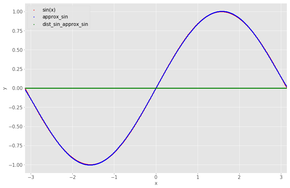
This is part of my goal to better understand linear algebra by working through the book Linear Algebra Done Right by Sheldon Axler. This notebook demonstrates how to approximate the sin(x) function by doing an orthogonal projection of the function onto the orthogonal basis of the inner product space with polynomial degree up to 5.
Intuitively, this can be understood as describing sin(x) as a linear combination of independent components (the orthonormal polynomials).
Why orthonormal basis?
Orthonormal basis has the following nice property: \(v = \langle v, e_0 \rangle e_0 + \langle v, e_1 \rangle e_1 + \ldots + \langle v, e_n \rangle e_n\) for any \(v \in V\) and the orthonormal basis \((e_0, e_1, \ldots, e_n)\). This means that we can find the coefficients for \(e_j\) in the linear combination by simply computing the inner product of \(v\) and \(e_j\). For a non-orthonormal basis, finding the coefficients is more difficult.
Why orthogonal projection as approximation?
Linear approximation by orthogonal projection onto the orthonormal basis ensures that the appoximation is optimal within the decided inner product subspace (i.e., solving a minimization problem). This comes from the proposition:
Suppose \(U\) is a subspace of \(V\) and \(v \in V\). Then \(||v - P_Uv|| \leq ||v-u||\)
for every \(u \in U\). Furthermore, if \(u \in U\) and the inequality above is an equality, then \(u = P_Uv\).
Note that here we require that \(v \in V\) and \(U \subseteq V\). This means that \(v\) is from a potentially larger inner product space and we are projecting \(v\) onto the \(U\) subspace. This is different from just representing \(v\) as a linear combination of the orthonormal basis of \(V\). Often, we do not know the inner product space that \(v\) comes from, or worse, \(dim V = \infty\), i.e., \(v\) comes from the infinite dimensional inner product space. By approximating $v$ in a finite dimensional subspace $U$, we lose the information about \(v\) for the parts that are not contained within subspace \(U\).
What are the use cases?
One of the many applications is when you have a function that you can evaluate but that you don’t know the exact form or if the exact form is too complicated to do any further manipulations, e.g., differentiation and integration.
Using the linear approximation of the function, you can configure the “complexity” of the approximation and also ensure that you get a “nice” function which can be easily manipulated by linear maps, e.g., differentiation and integration.
In the ML/DS domain, using a more simple linear approximation can also be motivated by the necessity of being able to generalize and not overfit the data.
Essential concepts
- Gram-Schmidt procedure: Transforms any basis to an orthonormal basis
- Orthonormal basis: each of the components in the basis are orthogonal to each other, i.e., \(\forall_{i, j \in {1, \dots, n} \wedge i \neq j} \text{inner product}(e_i, e_j) = 0\), and \(\forall_{1 \leq i \leq n} ||e_i|| = 1\)
Example from the book
# plot sin curve
s = 5

fig, ax = plt.subplots(figsize=(15, 10))

def approx_sin(x):
    return 0.987862 * x - 0.155271 * (x ** 3) + 0.00564312 * (x ** 5)

df = pd.DataFrame({'x': np.linspace(-np.pi, np.pi, 1000)})
df['sin(x)'] = df['x'].apply(np.sin)
df['cos(x)'] = df['x'].apply(np.cos)
df['approx_sin'] = df['x'].apply(approx_sin)
df.head()

# measure the distance between sin(x) and cos(x)
def dist(x, f, g):
    y_f = f(x)
    y_g = g(x)
    return abs(y_f - y_g) ** 2

df['dist_sin_cos'] = df['x'].apply(lambda x: dist(x, np.cos, np.sin))
df['dist_sin_approx_sin'] = df['x'].apply(lambda x: dist(x, np.sin, approx_sin))

# all
# curves = [ 'sin(x)', 'cos(x)', 'approx_sin', 'dist_sin_cos', 'dist_sin_approx_sin' ]
# colors = [ 'red', 'blue', 'purple', 'green', 'orange' ]

# sin and approx sin
curves = [ 'sin(x)', 'approx_sin', 'dist_sin_approx_sin' ]
colors = [ 'red', 'blue', 'green' ]

for curve, color in zip(curves, colors):
    df.plot(ax=ax, kind='scatter', x='x', y=curve, s=s,
            label=curve, color=color)

ax.set_ylabel('y')
ax.set_xlabel('x')

# set the xlim to -pi till pi
ax.set_xlim([-np.pi, np.pi]);

# define inner product function
def inner_product(f, g):
    return quad(lambda x: f(x) * g(x), -np.pi, np.pi)[0]
Approximate the sin curve using a 5 degree polynomial
Compute the orthonormal basis by applying the Gram-Schmidt procedure
# standard basis: (1, x, x**2, x**3, x**4, x**5)
normalize_e0 = np.sqrt(inner_product(lambda x: 1, lambda x: 1))
e0 = lambda x: 1 / normalize_e0

print('e0: {}'.format(normalize_e0))

ip_v1_e0 = inner_product(lambda x: x, e0)
f_e1 = lambda x: x - (ip_v1_e0 * e0(x))
normalize_e1 = np.sqrt(inner_product(f_e1, f_e1))
e1 = lambda x: f_e1(x) / normalize_e1

print('normalizing term e1: {}'.format(normalize_e1))

ip_v2_e0 = inner_product(lambda x: x**2, e0)
ip_v2_e1 = inner_product(lambda x: x**2, e1)
f_e2 = lambda x: x**2 - (ip_v2_e0 * e0(x)) - (ip_v2_e1 * e1(x))
normalize_e2 = np.sqrt(inner_product(f_e2, f_e2))
e2 = lambda x: f_e2(x) / normalize_e2

print('normalizing term e2: {}'.format(normalize_e2))

ip_v3_e0 = inner_product(lambda x: x**3, e0)
ip_v3_e1 = inner_product(lambda x: x**3, e1)
ip_v3_e2 = inner_product(lambda x: x**3, e2)
f_e3 = lambda x: x**3 - (ip_v3_e0 * e0(x)) - (ip_v3_e1 * e1(x)) \
    - (ip_v3_e2 * e2(x))
normalize_e3 = np.sqrt(inner_product(f_e3, f_e3))
e3 = lambda x: f_e3(x) / normalize_e3

print('normalizing term e3: {}'.format(normalize_e3))

ip_v4_e0 = inner_product(lambda x: x**4, e0)
ip_v4_e1 = inner_product(lambda x: x**4, e1)
ip_v4_e2 = inner_product(lambda x: x**4, e2)
ip_v4_e3 = inner_product(lambda x: x**4, e3)
f_e4 = lambda x: x**4 - (ip_v4_e0 * e0(x)) - (ip_v4_e1 * e1(x)) \
    - (ip_v4_e2 * e2(x)) - (ip_v4_e3 * e3(x))
normalize_e4 = np.sqrt(inner_product(f_e4, f_e4))
e4 = lambda x: f_e4(x) / normalize_e4

print('normalizing term e4: {}'.format(normalize_e4))

ip_v5_e0 = inner_product(lambda x: x**5, e0)
ip_v5_e1 = inner_product(lambda x: x**5, e1)
ip_v5_e2 = inner_product(lambda x: x**5, e2)
ip_v5_e3 = inner_product(lambda x: x**5, e3)
ip_v5_e4 = inner_product(lambda x: x**5, e4)
f_e5 = lambda x: x**5 - (ip_v5_e0 * e0(x)) - (ip_v5_e1 * e1(x)) \
    - (ip_v5_e2 * e2(x)) - (ip_v5_e3 * e3(x)) \
    - (ip_v5_e4 * e4(x))
normalize_e5 = np.sqrt(inner_product(f_e5, f_e5))
e5 = lambda x: f_e5(x) / normalize_e5

print('normalizing term e5: {}'.format(normalize_e5))
e0: 2.5066282746310002
normalizing term e1: 4.546520770897223
normalizing term e2: 7.375872796990425
normalizing term e3: 11.750342444180532
normalizing term e4: 18.603305279385573
normalizing term e5: 29.369218654739278
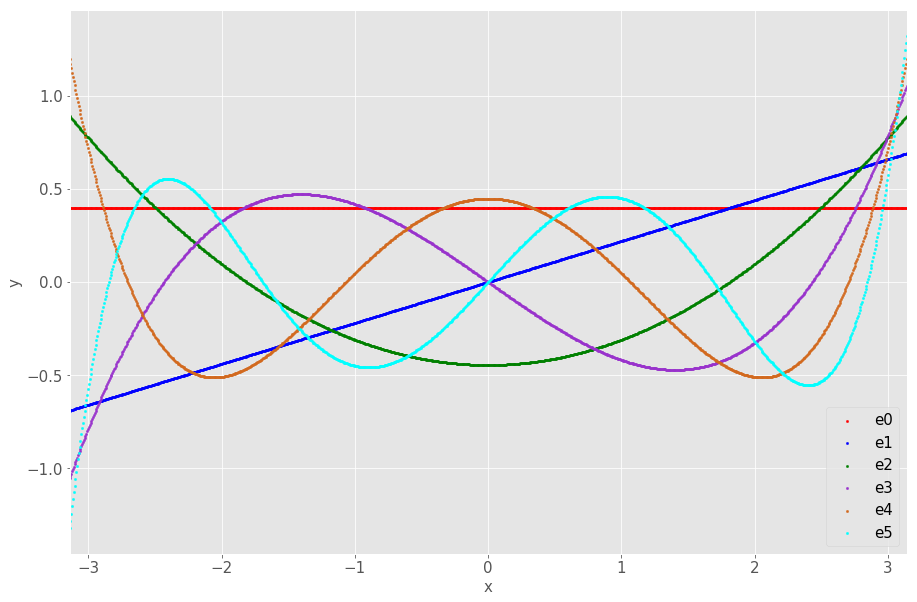
Visualize the orthonormal basis
# graph out the orthonormal bases
s = 5

fig, ax = plt.subplots(figsize=(15, 10))

xmin = -np.pi
xmax = np.pi
df = pd.DataFrame({'x': np.linspace(xmin, xmax, 1000)})
df['e0'] = df['x'].apply(e0)
df['e1'] = df['x'].apply(e1)
df['e2'] = df['x'].apply(e2)
df['e3'] = df['x'].apply(e3)
df['e4'] = df['x'].apply(e4)
df['e5'] = df['x'].apply(e5)

df.head()

curves = [ 'e0', 'e1', 'e2', 'e3', 'e4', 'e5' ]
colors = [ 'red', 'blue', 'green', 'darkorchid', 'chocolate', 'cyan' ]

for curve, color in zip(curves, colors):
    df.plot(ax=ax, kind='scatter', x='x', y=curve, s=s,
            label=curve, color=color)

ax.set_ylabel('y')
ax.set_xlabel('x')

# set the xlim to -pi till pi
ax.set_xlim([xmin, xmax]);

Approximating the sin(x) function by projecting it to a orthonormal basis of the polynomial inner product space of degree up to 5
This is easily achieved by using the linear combination properties of a orthonormal basis. Specifically, you would want a orthogonal projection since you can potentially represent a function in the infinite dimensional vector space, i.e., \(P_{\infty}(F)\).
Suppose you want to approximate function \(v(x)\) as a n-degree polynomial, then using projecting v onto the orthonormal basis of \(U = span(e_0, e_1, \ldots, e_n)\) would get: \(P_U(v) = \langle v, e_0 \rangle e_0 + \langle v, e_1 \rangle e_1 + \langle v, e_2 \rangle e_2 + \ldots + \langle v, e_n \rangle e_n\)
Closest possible approximation
Linear approximation by orthogonal projection onto the orthonormal basis also ensures that the appoximation is optimal (i.e., solving a minimization problem). This comes from the proposition:
Suppose \(U\) is a subspace of \(V\) and \(v \in V\). Then \(||v - P_Uv|| \leq ||v-u||\)
for every \(u \in U\). Furthermore, if \(u \in U\) and the inequality above is an equality, then \(u = P_Uv\).
Note that the approximation works even for functions in the infinite dimensional space (i.e., any vectors / polynomials) since we are limiting the approximation to a finite dimensional subspace.
# computing the coefficients of the linear combination
a_0 = inner_product(np.sin, e0)
a_1 = inner_product(np.sin, e1)
a_2 = inner_product(np.sin, e2)
a_3 = inner_product(np.sin, e3)
a_4 = inner_product(np.sin, e4)
a_5 = inner_product(np.sin, e5)

approx_sin_d0 = lambda x: a_0 * e0(x)
approx_sin_d1 = lambda x: a_0 * e0(x) + a_1 * e1(x)
approx_sin_d2 = lambda x: a_0 * e0(x) + a_1 * e1(x) + a_2 * e2(x)
approx_sin_d3 = lambda x: a_0 * e0(x) + a_1 * e1(x) + a_2 * e2(x) + \
    a_3 * e3(x)
approx_sin_d4 = lambda x: a_0 * e0(x) + a_1 * e1(x) + a_2 * e2(x) + \
    a_3 * e3(x) + a_4 * e4(x)
approx_sin_d5 = lambda x: a_0 * e0(x) + a_1 * e1(x) + a_2 * e2(x) + \
    a_3 * e3(x) + a_4 * e4(x) + a_5 * e5(x)
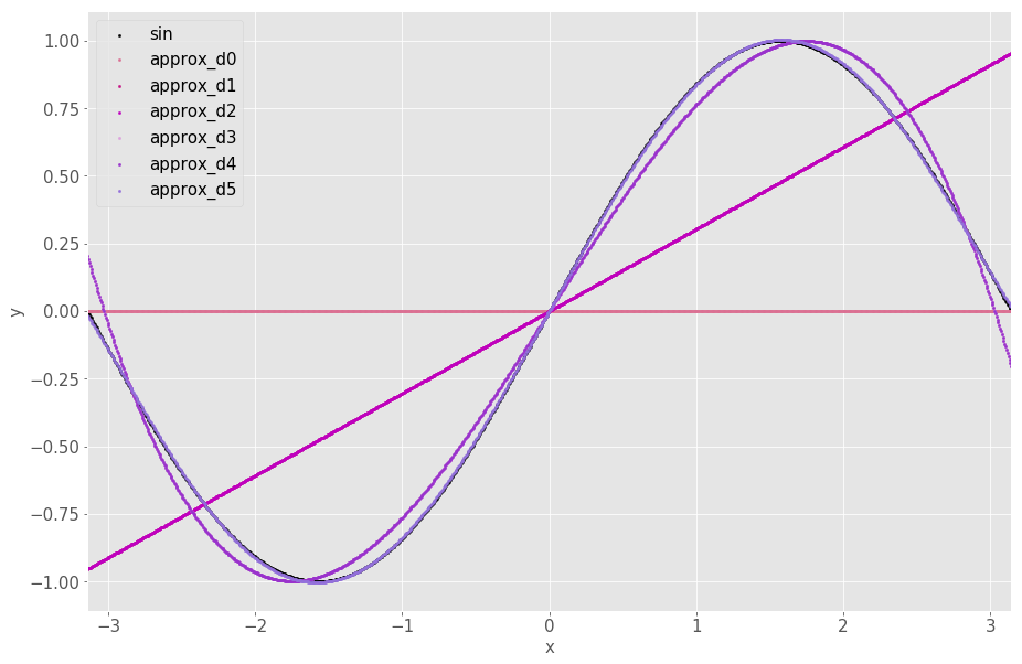
Visualizing the sin approximation and sin(x)
It shows that the approximation at 5 degree is so close to sin(x) that they are practically the same…
# graph out the orthonormal bases
s = 5

fig, ax = plt.subplots(figsize=(15, 10))

xmin = -np.pi
xmax = np.pi
df = pd.DataFrame({'x': np.linspace(xmin, xmax, 1000)})
df['sin'] = df['x'].apply(np.sin)
df['approx_d0'] = df['x'].apply(approx_sin_d0)
df['approx_d1'] = df['x'].apply(approx_sin_d1)
df['approx_d2'] = df['x'].apply(approx_sin_d2)
df['approx_d3'] = df['x'].apply(approx_sin_d3)
df['approx_d4'] = df['x'].apply(approx_sin_d4)
df['approx_d5'] = df['x'].apply(approx_sin_d5)
df.head()

curves = [ 'sin', 'approx_d0', 'approx_d1', 'approx_d2',
         'approx_d3', 'approx_d4', 'approx_d5']
colors = [ 'black', 'palevioletred',
          'mediumvioletred', 'm', 'plum', 'darkorchid', 'mediumpurple' ]


for curve, color in zip(curves, colors):
    df.plot(ax=ax, kind='scatter', x='x', y=curve, s=s,
            label=curve, color=color)

ax.set_ylabel('y')
ax.set_xlabel('x')

# set the xlim to -pi till pi
ax.set_xlim([xmin, xmax]);

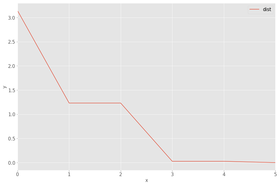
Measuring how quality of the approximation improves with the number of degree
Quality is measured by the following distance function between the approximation and sin(x): \(dist(sin, u) = \int^{-\pi}_{\pi} |sin(x) - u(x)|^2 dx\)
# measure the distance between sin(x) and cos(x)
def dist(f, g):
    return quad(lambda x: abs(f(x) - g(x)) ** 2, -np.pi, np.pi)[0]

# plot sin curve
s = 5

fig, ax = plt.subplots(figsize=(15, 10))

# map from degree to linear approximation
_f_map = {0: approx_sin_d0,
         1: approx_sin_d1,
         2: approx_sin_d2,
         3: approx_sin_d3,
         4: approx_sin_d4,
         5: approx_sin_d5}

df = pd.DataFrame({'degree': np.arange(0, 6)})
df['dist'] = df['degree'].apply(lambda m: dist(np.sin, _f_map[m]))

df.plot(kind='line', x='degree', y='dist', ax=ax)

ax.set_ylabel('y')
ax.set_xlabel('x');

The above figure shows that the quality of the approximation improves really quickly with distance reaching almost 0 with the linear approximation of degree 3 and very minor improvements using the linear approximation of degree 4 and 5.
Future exploration…
- try out other more interesting real-life functions.
- explore the connection with KL-divergence which is used to approximate probability distributions for Bayesian methods.
